Image Classification

Introduction

Motivation

Image Classification problem, which is the task of assigning an input image one label from a fixed set of categories. many other seemingly distinct Computer Vision tasks (such as object detection, segmentation) can be reduced to image classification.

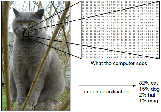
Example: image classification model takes a single image and assigns probabilities to 4 labels, {cat, dog, hat, mug}. an image is represented as one large 3-dimensional array of numbers.the cat image is 248 pixels wide, 400 pixels tall, and has three color channels Red,Green,Blue (or RGB for short). Therefore, the image consists of 248 x 400 x 3 numbers, or a total of 297,600 numbers. Each number is an integer that ranges from 0 (black) to 255 (white). Our task is to turn this quarter of a million numbers into a single label, such as “cat”.

Challenges

recognizing a visual concept (e.g. cat) is relatively trivial for a human to perform. keep in mind the raw representation of images as a 3-D array of brightness values:

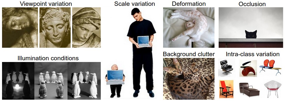
• Viewpoint variation. A single instance of an object can be oriented in many ways with respect to the camera.
• Scale variation. Visual classes often exhibit variation in their size (size in the real world, not only in terms of their extent in the image).
• Deformation. Many objects of interest are not rigid bodies and can be deformed in extreme ways.
• Occlusion. The objects of interest can be occluded. Sometimes only a small portion of an object (as little as few pixels) could be visible.
• Illumination conditions. The effects of illumination are drastic on the pixel level.
• Background clutter. The objects of interest may blend into their environment, making them hard to identify.
• Intra-class variation. The classes of interest can often be relatively broad, such as chair. There are many different types of these objects, each with their own appearance.

A good image classification model must be invariant to the cross product of all these variations, while simultaneously retaining sensitivity to the inter-class variations.

Solution

Data-driven approach. Unlike writing an algorithm for, for example, sorting a list of numbers, it is not obvious how one might write an algorithm for identifying cats in images. provide the computer with many examples of each class and then develop learning algorithms that look at these examples and learn about the visual appearance of each class. This approach is referred to as a data-driven approach, since it relies on first accumulating a training dataset of labeled images.

The image classification pipeline:

• Input: Our input consists of a set of N images, each labeled with one of K different classes. We refer to this data as the training set.
• Learning: Our task is to use the training set to learn what every one of the classes looks like. We refer to this step as training a classifier, or learning a model.
• Evaluation: In the end, we evaluate the quality of the classifier by asking it to predict labels for a new set of images that it has never seen before. We will then compare the true labels of these images to the ones predicted by the classifier. Intuitively, we’re hoping that a lot of the predictions match up with the true answers (which we call the ground truth).

Nearest Neighbor Classifier

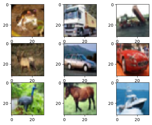
has nothing to do with Convolutional Neural Networks and it is very rarely used in practice but it is the most basic approach One popular toy image classification dataset is the CIFAR-10 dataset. This dataset consists of 60,000 tiny images that are 32 pixels high and wide. Each image is labeled with one of 10 classes (for example “airplane, automobile, bird, etc”) these 60,000 images are partitioned into a training set of 50,000 images and a test set of 10,000 images. The nearest neighbor classifier will take a test image, compare it to every single one of the training images, and predict the label of the closest training image. how we compare two images, which in this case are just two blocks of 32 x 32 x 3. One of the simplest possibilities is to compare the images pixel by pixel and add up all the differences. In other words, given two images and representing them as vectors I1,I2 , a reasonable choice for comparing them might be the L1 distance (for one color channel in this example)

evaluation criterion, it is common to use the accuracy, which measures the fraction of predictions that were correct. Notice that all classifiers we will build satisfy this one common API: they have a train(X,y) function that takes the data and the labels to learn from. Internally, the class should build some kind of model of the labels and how they can be predicted from the data. And then there is a predict(X) function, which takes new data and predicts the labels.

import numpy as np
from tqdm.notebook import trange


class NearestNeighborImageClassifier(object):
    def __init__(self):
        pass

    def train(self, X, y):
        """X is an N x M matrix where each row is an image. Y contains the labels for each image and is therefore 1 x N"""
        # the nearest neighbor classifier simply remembers all the training data
        self.trainX = X
        self.trainy = y

    def predict(self, X):
        """X is an N x M matrix where each row is an image we wish to predict a label for"""
        num_test = X.shape[0]
        # lets make sure that the output type matches the input type
        Ypred = np.zeros(num_test, dtype=self.trainX.dtype)

        # loop over all test rows
        for i in trange(num_test):
            # find the nearest training image to the i'th test image
            # using the L1 distance (sum of absolute value differences)
            distances = np.sum(np.abs(self.trainX - X[i, :]), axis=1)
            min_index = np.argmin(distances)  # get the index with smallest distance
            Ypred[i] = self.trainy[min_index]  # predict the label of the nearest example

        return Ypred

from matplotlib import pyplot
from keras.datasets import cifar10

(trainX, trainy), (testX, testy) = cifar10.load_data()
# summarize loaded dataset
print('Train: X=%s, y=%s' % (trainX.shape, trainy.shape))
print('Test: X=%s, y=%s' % (testX.shape, testy.shape))
# plot first few images
for i in range(9):
    pyplot.subplot(330 + 1 + i)
    pyplot.imshow(trainX[i])
# show the figure
pyplot.show()

2022-10-03 18:03:13.504284: I tensorflow/core/platform/cpu_feature_guard.cc:193] This TensorFlow binary is optimized with oneAPI Deep Neural Network Library (oneDNN) to use the following CPU instructions in performance-critical operations:  AVX2 FMA
To enable them in other operations, rebuild TensorFlow with the appropriate compiler flags.


Train: X=(50000, 32, 32, 3), y=(50000, 1)
Test: X=(10000, 32, 32, 3), y=(10000, 1)

nn = NearestNeighborImageClassifier()
trainX_rows = trainX.reshape(trainX.shape[0], 32 * 32 * 3)  # Xtr_rows becomes 50000 x 3072
testX_rows = testX.reshape(testX.shape[0], 32 * 32 * 3)  # Xte_rows becomes 10000 x 3072
nn.train(trainX_rows, trainy)
#Ypred = nn.predict(testX_rows) # predict labels on the test images
#print("accuracy: %f", np.mean(YpredTest == testy))

more impressive than guessing at random (which would give 10% accuracy since there are 10 classes), but nowhere near human performance (which is estimated at about 94%) or near state-of-the-art Convolutional Neural Networks that achieve about 95%. nother common choice could be to instead use the L2 distance, which has the geometric interpretation of computing the euclidean distance between two vectors. pixelwise difference as before, but this time we square all of them, add them up and finally take the square root this gives bigger differences more wheight. distances = np.sqrt(np.sum(np.square(self.Xtr - X[i,:]), axis = 1)) practical nearest neighbor application we could leave out the square root operation because square root is a monotonic function. That is, it scales the absolute sizes of the distances but it preserves the ordering, so the nearest neighbors with or without it are identical.

K - Nearest Neighbor Classifier

Also commonly reffered to as KNN

only use the label of the nearest image when we wish to make a prediction. Indeed, it is almost always the case that one can do better by using what’s called a k-Nearest Neighbor Classifier. The idea is very simple: instead of finding the single closest image in the training set, we will find the top k closest images, and have them vote on the label of the test image. In particular, when k = 1, we recover the Nearest Neighbor classifier. Intuitively, higher values of k have a smoothing effect that makes the classifier more resistant to outliers

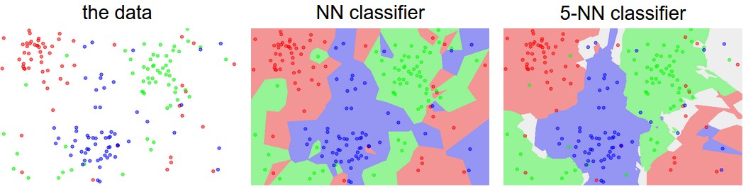
An example of the difference between Nearest Neighbor and a 5-Nearest Neighbor classifier, using 2-dimensional points and 3 classes (red, blue, green). The colored regions show the decision boundaries induced by the classifier with an L2 distance. The white regions show points that are ambiguously classified (i.e. class votes are tied for at least two classes). Notice that in the case of a NN classifier, outlier datapoints (e.g. green point in the middle of a cloud of blue points) create small islands of likely incorrect predictions, while the 5-NN classifier smooths over these irregularities, likely leading to better generalization on the test data (not shown).

what value of k should you use?

Hyperparameter Optimization

But what number works best? Additionally, we saw that there are many different distance functions we could have used: L1 norm, L2 norm. These choices are called hyperparameters.

You might be tempted to suggest that we should try out many different values and see what works best. That is a fine idea and that’s indeed what we will do, but this must be done very carefully. In particular, we cannot use the test set for the purpose of tweaking hyperparameters. Whenever you’re designing Machine Learning algorithms, you should think of the test set as a very precious resource that should ideally never be touched until one time at the very end. Otherwise, the very real danger is that you may tune your hyperparameters to work well on the test set, but if you were to deploy your model you could see a significantly reduced performance. In practice, we would say that you overfit to the test set. Another way of looking at it is that if you tune your hyperparameters on the test set, you are effectively using the test set as the training set, and therefore the performance you achieve on it will be too optimistic with respect to what you might actually observe when you deploy your model. But if you only use the test set once at end, it remains a good proxy for measuring the generalization of your classifier

The idea is to split our training set in two: a slightly smaller training set, and what we call a validation set. Using CIFAR-10 as an example, we could for example use 49,000 of the training images for training, and leave 1,000 aside for validation. This validation set is essentially used as a fake test set to tune the hyper-parameters.

valX_rows = trainX_rows[:1000, :]
valy = trainy[:1000]
trainX_rows = trainX_rows[1000:, :]
trainy = trainy[1000:]

# find hyperparameters that work best on the validation set
validation_accuracies = []
for k in [1, 3, 5, 10, 20, 50, 100]:
    #nn = NearestNeighbor()
    #nn.train(Xtr_rows, Ytr)
    # here we assume a modified NearestNeighbor class that can take a k as input
    #Yval_predict = nn.predict(Xval_rows, k = k)
    #acc = np.mean(Yval_predict == Yval)
    #print 'accuracy: %f' % (acc,)

    # keep track of what works on the validation set
    #validation_accuracies.append((k, acc))
    pass

Cross-validation

In cases where the size of your training data (and therefore also the validation data) might be small, people sometimes use a more sophisticated technique for hyperparameter tuning called cross-validation. instead of arbitrarily picking the first 1000 datapoints to be the validation set and rest training set, you can get a better and less noisy estimate of how well a certain value of k works by iterating over different validation sets and averaging the performance across these. For example, in 5-fold cross-validation, we would split the training data into 5 equal folds, use 4 of them for training, and 1 for validation.

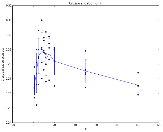
Example of a 5-fold cross-validation run for the parameter k. For each value of k we train on 4 folds and evaluate on the 5th. Hence, for each k we receive 5 accuracies on the validation fold. The trend line is drawn through the average of the results for each k and the error bars indicate the standard deviation. Note that in this particular case, the cross-validation suggests that a value of about k = 7 works best on this particular dataset (corresponding to the peak in the plot).

In practice, people prefer to avoid cross-validation in favor of having a single validation split, since cross-validation can be computationally expensive.

Pros and Cons of Nearest Neighbor classifiers

one advantage is that it is very simple to implement and understand. Additionally, the classifier takes no time to train, since all that is required is to store and possibly index the training data. However, we pay that computational cost at test time, since classifying a test example requires a comparison to every single training example. in practice we often care about the test time efficiency much more than the efficiency at training time. In fact, the deep neural networks we will develop later in this class shift this tradeoff to the other extreme: They are very expensive to train, but once the training is finished it is very cheap to classify a new test example. This mode of operation is much more desirable in practice.

The classifier must remember all of the training data and store it for future comparisons with the test data. This is space inefficient because datasets may easily be gigabytes in size.

a good choice in some settings (especially if the data is low-dimensional), but it is rarely appropriate for use in practical image classification settings. One problem is that images are high-dimensional objects (i.e. they often contain many pixels), and distances over high-dimensional spaces can be very counter-intuitive. Pixel-based distances on high-dimensional data (and images especially) can be very unintuitive. An original image (left) and three other images next to it that are all equally far away from it based on L2 pixel distance.